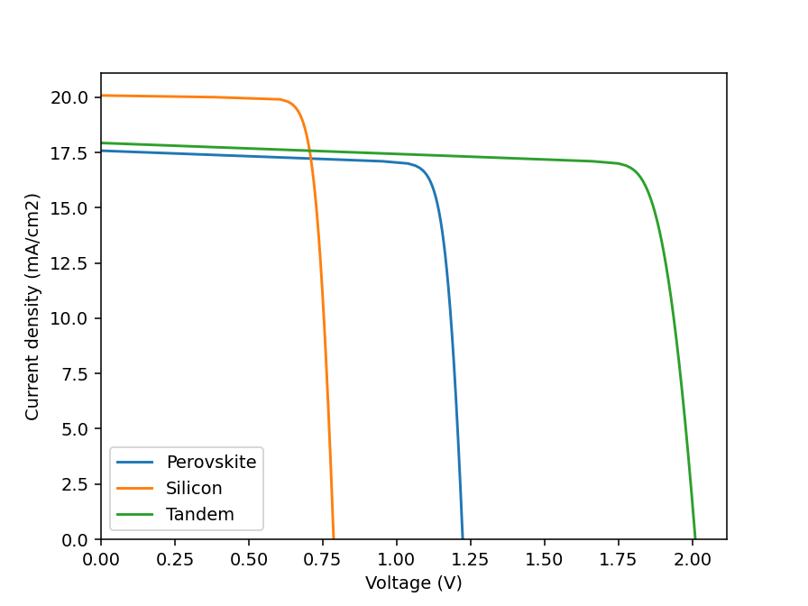
Tandem Solar Cell under STC

Simulating the IV curve of a Tandem Solar Cell with a 1-Diode model.

This example shows how to model the performance of a tandem solar cell. It uses “spectral-on-demand” data from the NSRDB providded by NREL. For the absorptances of the subcells GENPRO4 simulated EQE curves are used originally createf for the following publication: Reference ———- .. [1] P. Tillmann, K. Jäger, A. Karsenti, L. Kreinin, C. Becker (2022)

“Model-Chain Validation for Estimating the Energy Yield of Bifacial Perovskite/Silicon Tandem Solar Cells,” Solar RRL 2200079, DOI: 10.1002/solr.202200079

First, we load the preprocessed spectral and meta-data (for temperature) The spectral data has to be converted from W/µm/m2 to W/nm/m2 (by deviding by 1000)

import pandas as pd
import numpy as np
import matplotlib.pyplot as plt
from pv_tandem import utils, solarcell_models
import pvlib

plt.rcParams["figure.dpi"] = 140

eqe = pd.read_csv("./data/eqe_tandem_2t.csv", index_col=0)

Note that the airmass and zenith values do not exactly match the values in the technical report; this is because airmass is estimated from solar position and the solar position calculation in the technical report does not exactly match the one used here. However, the differences are minor enough to not materially change the spectra.

electrical_parameters = {
    "Rsh": {"pero": 2000, "si": 5000},
    "RsTandem": 3,
    "j0": {"pero": 2.7e-18, "si": 1e-12},
    "n": {"pero": 1.1, "si": 1},
    "Temp": {"pero": 25, "si": 25},
    "noct": {"pero": 48, "si": 48},
    "tcJsc": {"pero": 0.0002, "si": 0.00032},
    "tcVoc": {"pero": -0.002, "si": -0.0041},
}

tandem = solarcell_models.TandemSimulator2T(
    eqe=eqe,
    electrical_parameters=electrical_parameters,
    subcell_names=["pero", "si"],
)

iv_stc = tandem.calc_IV_stc()
fig, ax = plt.subplots()

for subcell, iv in iv_stc.items():
    iv = iv[(iv > 0).shift(1, fill_value=True)]
    iv = iv.reset_index().set_index(subcell)
    iv.plot(ax=ax)

ax.legend(["Perovskite", "Silicon", "Tandem"])
ax.set_xlabel("Voltage (V)")
ax.set_ylabel("Current density (mA/cm2)")
ax.set_xlim(0)
ax.set_ylim(0)
plt.show()

previous

Gallery

next

Tandem Solar Cell under STC