Basic examples of bifacial modeling

Showcasing basic examples for modeling of bifacial irradiance

Introduction

This example shows how to model the irradiance on a bifacial solar cell module, for some examples in Berlin, Germany. The examples are similiar to some of the main figures of the following publication

1

P. Tillmann, K. Jäger, A. Karsenti, L. Kreinin, C. Becker (2022) “Model-Chain Validation for Estimating the Energy Yield of Bifacial Perovskite/Silicon Tandem Solar Cells,” Solar RRL 2200079, DOI: 10.1002/solr.202200079

from pv_tandem import geo
import matplotlib.pyplot as plt
import numpy as np
import pvlib
import pandas as pd
import seaborn as sns

coord_berlin = dict(latitude =52.5, longitude =13.4)

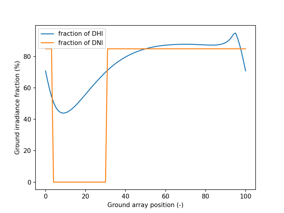
The geometry of the solar cell array and the sun position is defined. The ground between two rows is discretized into n elements, controlled by the parameter ground_steps and defaults to 101. The first example shows the distibution of irradiance of the direct and diffuse components on these 101 ground elements for a zenith angle of 31.0 deg and azimuth of 144.1 deg

vf = geo.ModuleIllumination(module_length=1.92,
    module_tilt=52,
    mount_height=0.5,
    module_spacing=7.3,
    zenith_sun=31.9,
    azimuth_sun=144.1,
    ground_steps=101)

fig, ax = plt.subplots(dpi=150)

ax.plot(vf.results['radiance_ground_diffuse_emitted']*np.pi*100)
ax.plot(vf.results['radiance_ground_direct_emitted']*np.pi*100)

ax.legend(['fraction of DHI', 'fraction of DNI'])

ax.set_ylabel('Ground irradiance fraction (%)')
ax.set_xlabel('Ground array position (-)')

plt.show()

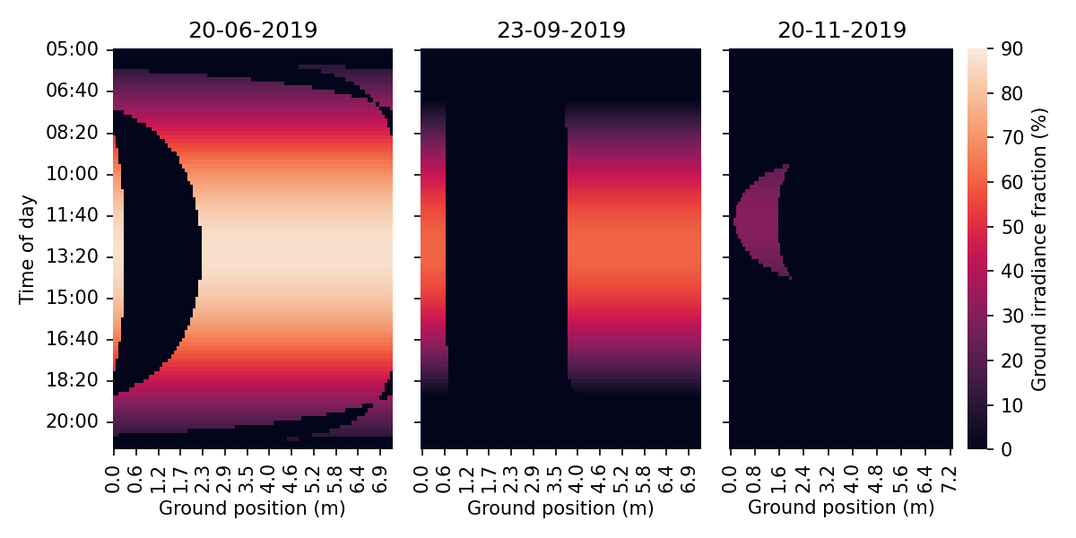
Next we look at how the evolution of the illumination develops during sommer solstice, equinox and winter solstice in Berlin. First the date ranges are defined and the python library pvlib is used to calculate the solar position (zenith and azimuth angle). For each of these days the ground illumination is calucated the the radiance is converted to irradiance by multipling with pi.

dt_list = [
    pd.date_range("20190620 5:00","20190620 21:00", freq='10min', tz='Europe/Berlin'),
    pd.date_range("20190923  5:00","20190923 21:00", freq='10min', tz='Europe/Berlin'),
    pd.date_range("20191120  5:00","20191120 21:00", freq='10min', tz='Europe/Berlin')]

fig, axes = plt.subplots(1,3,dpi=150, figsize=(8,4), sharey=True)
dates = ["20-06-2019", "23-09-2019", "20-11-2019"]

for i, dt in enumerate(dt_list):
    solar_pos = pvlib.solarposition.get_solarposition(dt, **coord_berlin)
    vf = geo.ModuleIllumination(module_length=1.92,
        module_tilt=52,
        mount_height=0.5,
        module_spacing=7.3,
        zenith_sun=solar_pos['zenith'],
        azimuth_sun=solar_pos['azimuth'],
        ground_steps=101,
        module_steps=12,
        angle_steps=180,)

    df_rgde = pd.DataFrame(vf.results['radiance_ground_direct_emitted']*np.pi*100,
                           index = dt.strftime("%H:%M"),
                           )
    df_rgde.columns = (vf.dist*df_rgde.columns / len(df_rgde.columns)).to_series().round(1)

    ax = axes[i]
    sns.heatmap(df_rgde,
                ax = ax,
                cbar = i>=2,
                yticklabels=10,
                vmin=0, vmax=90,
                )

    ax.set_xlabel("Ground position (m)")
    if i == 0:
        ax.set_ylabel("Time of day")

    ax.set_title(dates[i])

    if i >=2:
        ax.collections[0].colorbar.set_label('Ground irradiance fraction (%)')


fig.tight_layout()
plt.show()

/home/docs/checkouts/readthedocs.org/user_builds/pv-tandem/checkouts/stable/pv_tandem/bifacial_geo.py:89: UserWarning: Zenith angle larger then 90 deg was passed to simulation. Zenith angle is truncted to 90.
  warnings.warn(
/home/docs/checkouts/readthedocs.org/user_builds/pv-tandem/checkouts/stable/pv_tandem/bifacial_geo.py:89: UserWarning: Zenith angle larger then 90 deg was passed to simulation. Zenith angle is truncted to 90.
  warnings.warn(

The last example demonstrates the inhomogenity of the irradiance on the front and backside along the length of the PV module. The number of points for which the irradiance is evaluated along the module is ocntrolled by the parameter module_steps and defaults to 12.

vf = geo.ModuleIllumination(module_length=1.92,
    module_tilt=52,
    mount_height=0.5,
    module_spacing=7.3,
    zenith_sun=31.9,
    azimuth_sun=144.1)

sky_keys = ['irradiance_module_front_sky_direct',
 'irradiance_module_front_sky_diffuse',
 'irradiance_module_back_sky_direct',
 'irradiance_module_back_sky_diffuse']

ground_keys = ['irradiance_module_front_ground_direct',
    'irradiance_module_front_ground_diffuse',
    'irradiance_module_back_ground_direct',
    'irradiance_module_back_ground_diffuse']

legend_1 = ["front direct", "front diffuse", "back direct", "back diffuse"]
legend_2 = ["back direct", "back diffuse", "back direct", "back diffuse"]


fig, (ax1, ax2) = plt.subplots(2, figsize=(6,6), dpi=150, sharex=True)

for key in sky_keys:
    ax1.plot(vf.l_array, vf.results[key])

for key in ground_keys:
    ax2.plot(vf.l_array, vf.results[key])

ax1.set_ylabel('Irradiance fraction (%)')
ax1.legend(legend_1)
ax2.set_ylabel('Irradiance fraction (%)')
ax2.set_xlabel('Position on module (m)')
ax2.legend(legend_2)

<matplotlib.legend.Legend object at 0x7f31991fbf40>

previous

Tandem Solar Cell under STC

next

Energy Yield for Bifacial Tandem Solar Cell